 The Summarize Nearby tool finds features that are within a specified distance of features in the input layer using a line distance or travel mode. Statistics are then calculated for the nearby features.
Workflow diagram

Examples
A school board is building a new elementary school and needs to decide between several potential locations. They decide that the school should be in the area with the most children aged 5 to 12. The population of children aged 5 to 12 can be calculated with the Summarize Nearby tool using a one-mile walking distance around each potential location and census blocks that include population data.
Terminology
| Term | Description |
|---|---|
Geodesic | Refers to a line drawn on a sphere. A geodesic line drawn on the globe represents the curvature of the earth's geoid. |
Euclidean distance | A straight-line distance as measured on a flat surface (that is, a Cartesian plane). |
Usage notes
The Summarize Nearby tool requires two input layers: a layer from which distances will be measured and a layer to summarize. Both layers may be points, lines, or areas. The first input layer can contain up to 1,000 features.
The nearby distance can be based on a line distance or several different travel modes using time or distance as the measure. Travel modes are only enabled when the first input layer contains point features. You can create multiple output areas by inputting each time or distance separated by a space.
Some travel modes have an option for using traffic conditions. When traffic conditions are used, they may be based on live conditions or typical conditions for a specified day of the week and time. Live traffic conditions can be offset up to 12 hours from the current time. Times for typical conditions can be set by 15-minute intervals for the entire day and night.
Travel modes can be configured by the administrator of your organization. The administrator can also add new travel modes or remove travel modes that are not necessary for your organization. The default distance measure will be in Miles or Kilometers, depending on the Units setting in your profile.
| Travel Modes | Description | Defaults | Options |
|---|---|---|---|
| Follows paths and roads that allow pedestrian traffic and finds solutions that optimize travel time. The walking speed is set to 5 kilometers per hour. | Walking speed is set at 5 kilometers (3.1 miles) per hour. The walking speed can be configured by the administrator of your organization. The default Walking Time is 5 Minutes. | A duration of up to 5 hours can be used as input. Durations can be in Seconds, Minutes, or Hours. |
| Models the movement of cars and other similar small automobiles, such as pickup trucks, and finds solutions that optimize travel distance. Travel obeys one-way roads, avoids illegal turns, and follows other rules that are specific to cars but does not discourage travel on unpaved roads. | The default Rural Driving Distance is 5 Miles (US Standard setting) or 5 Kilometers (Metric setting). | A distance of up to 300 miles (482.80 kilometers) can be used as input. Distances can be in Miles, Yards, Feet, Kilometers, or Meters. |
| Models the movement of cars and other similar small automobiles, such as pickup trucks, and finds solutions that optimize travel time. Travel obeys one-way roads, avoids illegal turns, and follows other rules that are specific to cars. Dynamic travel speeds based on traffic are used where it is available when you specify a start time. Verify whether traffic data is available in your region by clicking the See availability link in the tool pane. | The default Driving Time is 5 Minutes. Use traffic is unchecked by default. The driving speed will be based on historical and live traffic data. | A duration of up to 5 hours can be used as input. Durations can be in Seconds, Minutes, or Hours. Traffic can be based on live conditions or typical conditions for a specified day of the week and time. |
| Models the movement of cars and other similar small automobiles, such as pickup trucks, and finds solutions that optimize travel distance. Travel obeys one-way roads, avoids illegal turns, and follows other rules that are specific to cars. | The default Driving Distance is 5 Miles (US Standard setting) or 5 Kilometers (Metric setting). | A distance of up to 300 miles (482.80 kilometers) can be used as input. Distances can be in Miles, Yards, Feet, Kilometers, or Meters. |
| Follows paths and roads that allow pedestrian traffic and finds solutions that optimize travel distance. | The default Walking Distance is 5 Miles (US Standard setting) or 5 Kilometers (Metric setting). | A distance of up to 300 miles (482.80 kilometers) can be used as input. Distances can be in Miles, Yards, Feet, Kilometers, or Meters. |
| Models the movement of cars and other similar small automobiles, such as pickup trucks, and finds solutions that optimize travel time. Travel obeys one-way roads, avoids illegal turns, and follows other rules that are specific to cars but does not discourage travel on unpaved roads. Dynamic travel speeds based on traffic are used where it is available when you specify a start time. Verify whether traffic data is available in your region by clicking the See availability link in the tool pane. | The default Rural Driving Time is 5 Minutes. Use traffic is unchecked by default. The rural driving speed will be based on historical and live traffic data. | A duration of up to 5 hours can be used as input. Durations can be in Seconds, Minutes, or Hours. Traffic can be based on live conditions or typical conditions for a specified day of the week and time. |
| Models basic truck travel by preferring designated truck routes and finds solutions that optimize travel time. Routes must obey one-way roads, avoid illegal turns, and so on. The trucking speed will be based on either historical average speeds for automobiles or the posted speed limits for trucks, whichever is smaller. Follows rules applicable to heavy trucks. | The default Trucking Time is 5 Minutes. | A duration of up to 5 hours can be used as input. Durations can be in Seconds, Minutes, or Hours. |
| Models basic truck travel by preferring designated truck routes and finds solutions that optimize travel distance. Routes must obey one-way roads, avoid illegal turns, and so on. Follows rules applicable to heavy trucks. | The default Trucking Distance is 5 Miles (US Standard setting) or 5 Kilometers (Metric setting). | A distance of up to 300 miles (482.80 kilometers) can be used as input. Distances can be in Miles, Yards, Feet, Kilometers, or Meters. |
The Return bounding areas box is checked by default. The result layer will include the area or areas created using the specified distance measurement around the input layer as well as all of the requested summarized data. When unchecked, the result layer will be the same as the input layer but include the summarized data.
A Count of Points, Total Length, or Total Area box will appear depending on the type of features to summarize in your layer. The boxes are checked by default and can only be unchecked if statistics are being calculated.
| Calculation | Input Features | Default | Options |
|---|---|---|---|
Count of Points | Points | None | None |
Total Length | Lines | Miles (US Standard setting) or Kilometers (Metric setting) |
|
Total Area | Areas | Square Miles (US Standard setting) or Square Kilometers (Metric setting) |
|
There are five options for statistics that can be calculated on numeric fields in the layer to be summarized: sum, minimum, maximum, average, and standard deviation. Each time a Field and Statistic is entered, a new row will be added to the tool pane so that more than one statistic can be calculated at once. The summarized data can be viewed in the result layer's table or pop-ups.
Optionally, a group field can be selected so statistics are calculated separately for each unique attribute value. When a group field is selected, the pop-up for each of the features in the output layer will contain charts showing each summary count or total and statistic by field value. A summary table listing each feature and statistic by group field value will also be created.
The Add minority, majority and Add percentages boxes are enabled when a group field is entered. The minority and majority will be the least and most dominant value from the group field, respectively, where dominance is determined using the count of points, total length, or total area of each value. When Add minority, majority is checked, two new fields will be added to the result layer. The fields will list the values from the group field that are the minority and majority for each result feature. When Add percentages is checked, two new fields will be added to the result layer listing the percentage of the count of points, total length, or total area that belong to the minority and majority values for each feature. A percentage field will also be added to the result table listing the percentage of the count of points, total length, or total area that belong to all values from the group field for each feature.
If Use current map extent is checked, only the features in the input layer and the layer to be summarized that are visible within the current map extent will be analyzed. If unchecked, all features in both the input layer and the layer to be summarized will be analyzed, even if they are outside the current map extent.
Limitations
- The first input layer from which distances are measured has a limit of 1,000 features.
- Travel modes will only be enabled when point features are used as the input layer from which distances are measured.
- Lines and areas are summarized using proportions; therefore, it is best to summarize absolute data (such as population) rather than relative data (such as average income) when lines or areas are being summarized.
How Summarize Nearby works
Equations
Average and Std Deviation are calculated using weighted mean and weighted standard deviation for line and area features. None of the statistics for point features are weighted. The following table shows the equations used to calculate standard deviation, weighted mean, and weighted standard deviation.
| Statistic | Equation | Variables | Features |
|---|---|---|---|
Standard Deviation |  |  | Points |
Weighted Mean |  |
| Lines and Areas |
Weighted Standard Deviation |  |
| Lines and Areas |
Points
Point layers are summarized using only the point features within the boundary drawn by the Summarize Nearby tool. If Return bounding areas is checked, the results layer will be displayed using graduated symbols.
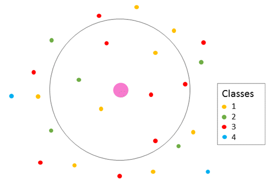
The figure and table below explain the statistical calculations of a point layer. In the hypothetical analysis in the figure, a point layer is being summarized using a line distance from an input point. The Classes field was used to calculate the statistics (Sum, Minimum, Maximum, Average, and Std Deviation) for the layer.

| Statistic | Result |
|---|---|
Sum | |
Minimum | Minimum of : |
Maximum | Maximum of : |
Average | |
Std Deviation |  |
A real-life scenario in which this analysis could be used is in determining the availability of yoga classes within a two-mile radius of your house. Each point represents a gym or studio that offers yoga classes. The Classes field gives the number of unique classes offered at each point. From the results, you can see that there are seven facilities offering classes within two miles of your house and that the maximum number of unique classes at a single facility is three.
Lines
Line layers are summarized using only the proportions of the line features that are within the boundary drawn by the Summarize Nearby tool. When summarizing lines, use fields with absolute numbers so proportional calculations make logical sense in your analysis. If Return bounding areas is checked, the results layer will be displayed using graduated symbols.
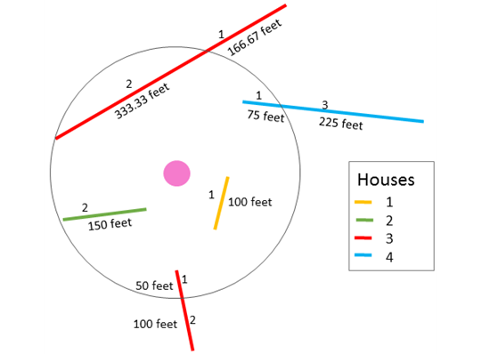
The figure and table below explain the statistical calculations of a line layer. In the hypothetical analysis in the figure, a line layer is being summarized using a line distance from an input point. The Houses field was used to calculate the statistics (Sum, Minimum, Maximum, Average, and Std Deviation) for the layer. The statistics are calculated using only the proportion of the line that is within the specified distance of the input point.

| Statistic | Result |
|---|---|
Sum | |
Minimum | Minimum of : |
Maximum | Maximum of : |
Average |  |
Std Deviation |  |
A real-life scenario in which this analysis could be used is in determining how many houses are within five miles of a remote forest fire. Each line segment represents a street or lane with houses built along it. The Houses field gives the number of houses on each segment. From the results, you can see that there are seven houses within five miles of the fire.
Areas
Area layers are summarized using only the proportions of the area features that are within the boundary drawn by the Summarize Nearby tool. When summarizing areas, use fields with absolute numbers so proportional calculations make logical sense in your analysis. If Return bounding areas is checked, the results layer will be displayed using graduated colors.
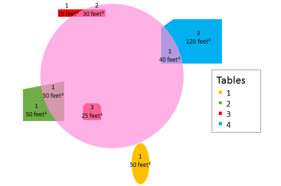
The figure and table below explain the statistical calculations of an area layer. In the hypothetical analysis in the figure, an area layer is being summarized using a line distance from an input point. The Tables field was used to calculate the statistics (Sum, Minimum, Maximum, Average, and Std Deviation) for the layer. The statistics are calculated using only the proportion of the area that is within the specified distance of the input point.

| Statistic | Result |
|---|---|
Sum | |
Minimum | Minimum of: |
Maximum | Maximum of: |
Average |  |
Std Deviation |  |
A real-life scenario in which this analysis could be used is in determining how many picnic tables there are within a 100-foot radius of different campsites. Each area represents a picnic site and the Tables field gives the number of picnic tables in each. From the results, you can see that there are seven tables near this specific campsite and the most picnic tables at a single site is three.
Line distance
The Summarize Nearby tool uses a geodesic method when finding features with a straight-line distance, rather than a Euclidean method. Geodesic lines account for the actual shape of the earth (an ellipsoid, or more properly, a geoid). Distances are calculated between two points on a curved surface (the geoid) as opposed to two points on a flat surface (the Cartesian plane).
Travel modes
Service Areas use Dijkstra's algorithm to traverse a network. The service returns a subset of connected edge features that are within a specified travel distance or travel time. Travel areas are created by inputting the edges into a triangulated irregular network (TIN) data structure. The network distance along the lines serves as the height of the locations inside the TIN. Locations not traversed by the service area are put in with a much larger height value. An area-generation routine is used with this TIN to carve out regions encompassing areas in between the specified break values (travel time or travel distance).
The Live traffic option uses the current time as the departure. The traffic speed is predicted for the trip using live speeds, historical speeds, and current events, such as weather.
When typical conditions for a day of the week and time are being used, the travel speeds are based on historical speeds averaged across 5-minute intervals for the entire week. The selected time will correspond to local time in the time zone that your data is in.
When either traffic condition is used, the Summarize Nearby tool will take into consideration the changing traffic conditions based on elapsed time from departure.
Similar tools
Use Summarize Nearby to calculate statistics on point, line, or area features within close proximity of another input layer. Other tools may be useful in solving similar but slightly different problems.
Map viewer analysis tools
If you have predefined boundaries in which you want to summarize a point, line, or area layer, use the Summarize Within tool.
If you have predefined boundaries in which you would like to summarize a point layer and you want to keep only the areas containing one or more points, use the Aggregate Points tool.
ArcGIS Desktop analysis tools
Summarize Nearby is also available in ArcGIS Pro. To run the tool from ArcGIS Pro, your project's active portal must be running Portal for ArcGIS 10.5 or later. You must also sign in to the portal using an account that has privileges to perform standard feature analysis in the portal.


